
A blog post by Fatih Ozturk.
Having an imbalanced dataset is one of the critical problems of machine learning algorithms. This is only valid for supervised learning cases, and also mostly for binary classification (0 or 1) cases.
At UrbanStat, we spend a lot of time working on these types of datasets due to the nature of insurance problems.
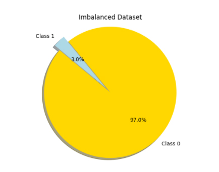
What is an imbalanced dataset?
It is the dataset where the number of instances in one class outnumbers the number of instances in other class by large amounts. For a manufacturing facility, there can be 30 defective products per 1000 products manufactured. In this case, we can think of there are 30 instances of class 1 and 970 instances of class 0. In real life, it’s easy to see examples of this situation.
Following examples are the most popular ones:
- Credit card fraud detection
- Cancer disease detection
- Defective product detection
- Customer churn detection
Data scientists interested in insurance sector are also affected by these types of datasets. Simply, when it comes to a claim prediction study among insurance policies, the ratio of policies having claims to all policies is usually between 0.02 and 0.06. That is, when you start to deal with insurance datasets you need to be ready to deal with imbalanced data.
Machine Learning Algorithms vs Imbalanced Datasets
Most of the classifiers are subjected to the accuracy of all their predictions during learning. At each iteration, the decrease in error of overall predictions is calculated. Therefore, for a classifier constructed from such data, it’s expected to see ‘Class 0’ for all predictions with a high probability. In other words, because if you say ‘no claim’ for all policies of an insurance company, your predictions will have an about 98% accuracy, which looks amazing indeed. However, none of the policies having claims is caught and when it comes to ‘houses in high crime area with no security alarms’ predictions this topic requires to be more and more cautious. Predicting all ‘positive’ classes (Class 1) as ‘negative’ class (Class 0) will result in some catastrophes otherwise.
Strategies
1.Resampling
Resampling is one of the most utilized approaches for this issue. There are different types of resampling methods, but we’re going to mention about three of them, which are the main ones.
Oversampling means increasing number of minority class(Class 1). For predicting whether there will be a claim in an insurance policy, let’s assume there are 990 policies with no claim (Class 0) and 10 policies with a claim (Class 1) in training data. Oversampling can be done by replicating observations of Class 1 with or without replacement in order to balance data. For our example, we should replicate 10 policies till reaching 990 in total. For Python coding, ‘resample’ utilities from ‘sklearn.utils’ module really facilitates this process.
Following code can be used to oversample any minority data with replacement.
from sklearn.utils import resample
minority_oversampled = resample(minority, replace=True, n_samples=990)
Unlikely to oversampling, undersampling approach deals with only majority class. It reduces the number of instances belonging to majority class and particularly used for datasets having really really much majority class observations.
For our example, it can be done by the following code.
majority_undersampled = resample(majority, replace=False, n_samples=10)
However, by undersampling, we literally lose information used for training. In the current example, we’ve lost 980 types of policies having no claim information. In order to eliminate downsides of undersampling, the number of undersampled data can be tried step by step, which is like a series of [500,200,100,50..] in our example. It doesn’t have to be equal to the number of minority class always. It can stop at different optimal points for different data.
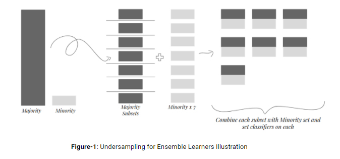
Another way to get rid of information loss is setting ensemble learners based on undersampled data. That is, for our example, there can be new 99 majority_subsets having 10 observations obtained by undersampling main majority class with replacement. Then, for each majority_subset minority observations are combined with them and 99 classifiers set on this combined subsets one by one. Finally, max voting criterion can be used to specify our final predictions.
SMOTE is a widely used resampling technique. SMOTE stands for ‘Synthetic Minority Oversampling Technique’. As the name of it implies, minority class is oversampled by creating a synthetic data in this method. In brief, SMOTE algorithm adds new observations having slightly different feature values from original observations and during calculations it utilizes each observations’ k-nearest neighbors. Those who want to learn more about the algorithm behind SMOTE can give a check on the reference [1].
Last but not least, all resampling operations have to be applied on only training datasets. Neither validation nor test datasets shouldn’t be resampled since such operations would result in unreliable model outcomes. By keeping these datasets clear off of these type of operations and monitoring prediction results on them, you can easily understand if resampling operations improved the model or not.
2.Using Class Weights
There are some classifiers which can be dictated class weights during learning such as Xgboost and RandomForest. Since classifiers try to minimize overall error during learning, they are biased to lower error of Class 0 while keeping error of Class 1 quite high, which is the minority class. When class weights come to play, classifiers tend to decrease error of class having a higher weight. For many classifiers default class weights are assigned as 1 and it’s best to start giving weights inversely proportional to the number of classes.
For our insurance claim prediction example, we have 990 observations for class 0 and 10 observations for class 1. So it’s quite appropriate to give class weights as 0.010 and 0.990 respectively. After this point, the weight of minority class might be altered until having satisfying results based on the objective.
Codes below are shown as an example of usage of class weights attribute in a Random Forest classifier in Python programming.
rf_classifier = RandomForestClassifier(n_estimators=80, class_weight={0: 0.01, 1: 0.99})
rf_classifier.fit(train[predicting_features], classes)
3. Using Correct Performance Parameters
Now we all know well that looking overall accuracy is a really bad way of evaluating a classifier set on an imbalanced data. Therefore, it’s critical to check correct performance parameters after each model result. Following are the most known correct performance parameters: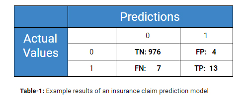
- Precision: How precisely do your 1 predictions hit real 1s?
- It’s calculated as TP/ (TP+FP) = 13/(4+13) = 0.77
- Recall: How much of real 1s are covered up by your 1 predictions?
- It’s calculated as TP/ (TP+FN) = 13/(7+13) = 0.65
- F1-Score: It’s a parameter calculated by some mathematical combinations of precision and recall.
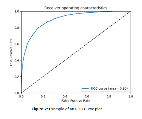
- ROC Curve: This curve and AUC (area under the curve) are used to show and measure how well model predictions distinguish two classes. For random predictions, AUC takes the value of 0.50. That is, any model that claims ‘deriving meaningful patterns from data’ has to have higher AUC values than 0.50.
References
[1] Chawla, N.V., Bowyer, K.W., Hall, L.O., Kegelmeyer W.P.: SMOTE: Synthetic Minority Over-Sampling Technique. Journal of Artificial Intelligence Research 16 (2002) 321-357