Insights

A blog post by Fatih Ozturk & Fatma Sen

Policy and claim file details are the most important datasets insurance carriers collect over the years. Policy datasets have dozens of features that contain important information like policy start/end dates, building info, location, premium, and other descriptive points that define risk. Claim datasets describe the events that caused damages to the covered entity and their financial outcomes. Building a predictive model using these datasets only usually fails to predict the likelihood of a claim for a given policy. Having flood claims in a region doesn’t mean that region has a statistically significant high flood risk as just not having flood claims in a region doesn’t mean that region has a statistically significant low flood risk. This is one of the simplest reasons for insurance carriers to use external datasets that could explain different phenomena (cat and non-cat events).

Not all claims are created equally

Claim prediction models cannot be as successful as labeling an image as ‘cat’ or ‘dog’ due to the nature of events that causes claims. All events have unique outputs and even the same type of events (e.g. floods) can have different underlying causes and entirely different outputs based on time, location, and infrastructure. Therefore, having only building related features and city/district information is not sufficient for satisfactory predictive power.

As UrbanStat has been targeting P&C lines that focus on buildings and liabilities caused by events that affect buildings, or their users, it only makes sense to use more ‘spatial’ features that can add further value against damage types.

Types of external datasets

At UrbanStat, we use datasets from 2 different type of sources:

• Private data partners
• Public organizations

Before we decide on which datasets to use for an insurance carrier, we do a preliminary analysis on claim distributions. For example, in Florida, most of the damage types belong to water-induced and wind-induced causes. So we pay more attention to sourcing risk datasets related to water, flood, storm, and hurricanes.  On the other hand, when looking at other regions these datasets are not as useful, so our focus is on snowfall, hail, and storms when it comes to modeling in Massachusetts.

Bringing in more datasets doesn’t guarantee the success, cleansing and processing those datasets are equally important. Before doing any kind of modeling, we focus on data cleansing and derivative data creation. For example, FEMA Flood Maps may have topographic errors or erroneous inputs but doesn’t require creating derivative datasets.

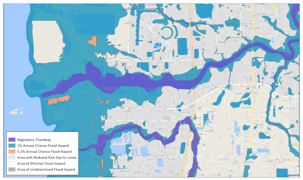
City of Tampa, Florida – FEMA Flood hazard map

Shoreline data itself doesn’t explain anything but by creating proximity maps as seen below we added enormous value to the claim prediction.

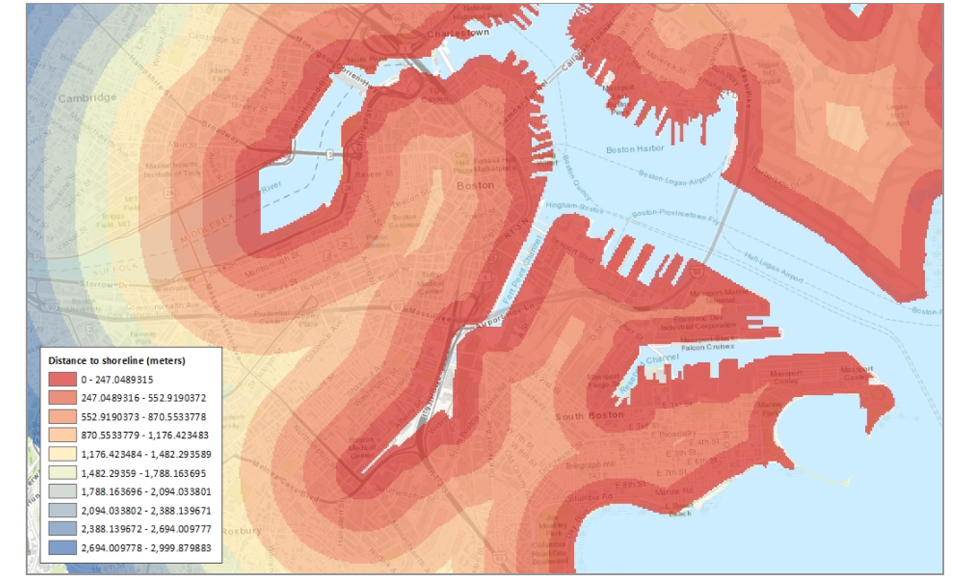
City of Boston, Massachusetts – Shoreline Proximity Map

Getting an edge

We have seen remarkable differences in our models when we used external datasets.  While it is really hard to have financially successful prediction results with datasets only provided by insurance companies, adding external datasets give much better prediction results and hence satisfactory financial improvements. Historically, 70 out of top 100 important features having an impact on financially successful predictions are actually the features UrbanStat has engineered.

Conclusion

The importance of bringing in new datasets in claim prediction is but one piece of the puzzle, really digging in and understanding which datasets can provide the most value for a specific purpose and then have the expertise to frame, build and design prediction models for each use case is where real impact occurs and where unexpected results are discovered. UrbanStat has continued to refine its models for all types of global geographies and business lines and continues to produce actionable results for its partners.

To learn more and quickly leverage what we’ve already successfully deployed for our carrier partners contact us at [email protected].

A blog post by Fatih Ozturk, Matt Carstens & Anil Celik

A couple of years ago when UrbanStat first started operating, our solutions focused on simulations, deterministic/probabilistic risk analysis, and data visualization. Leveraging a large list of external cat/non-cat data sets and having access to historical datasets from multiple insurance companies enabled us to focus more on machine learning based predictive analytics and create even more value for our carrier partners.

Our focus was on finding a way to accurately predict high-risk clients, at the time of underwriting, based on their likelihood of claims and damages within a year. Defining “high-risk” is very much dependent on the insurer’s risk appetite as the events we are trying to predict are quite rare and can materially affect the underwriters’ performance. This makes this problem both challenging and exciting as we’ve returned clear risk selection improvements with our partners.

The graph below visually communicates our goal and value-add in the risk selection process

All insurance carriers have this hypothetical curve (green zone) that represents the ideal clients they want to win. They are OK with paying claims, as long as they are in the green zone (risk appetite). However, carriers end up with this triangle instead (green + blue + red) due to common risk identifying complexities and the lack of proper tools (technology, skillset, team, process etc.) for this problem. Although it’s possible to identify many of the clients that are in the blue zone, It’s almost impossible to identify the ones in the red zone (or as we call internally the god-zone).

Every client is different so are their risks

We believe one of the most obvious reasons for missing “right” clients or winning “wrong” clients in the selection process is that carriers are still not granular enough in their segmentation. The problem with this type of segmentation is that many times clients are considered to be similar (if not identical) to everyone else in, let’s say, a given neighborhood so we need to come up with new approaches to enable personalized underwriting.

Automating a personalized risk selection process for an underwriting team is something we continue to refine and work with our carrier partners on. We continue to focus on identifying high-risk clients that are in the blue section in the graph above so insurance carriers can identify, reconsider or reject clients that pose a greater risk threshold than their internal mandates – as this small percentage of clients are actually threatening the wellness of the portfolio as a whole.

How to choose policies to be rejected?

At first glance, one may think it’s an easy question. You should reject policies that are more likely to have higher (how high is defined by the risk appetite) damages than their premiums, which are causing losses to companies. However, when this issue comes to ML, it’s not that easy.

Let’s assume there is an insurance company X and its main goal of ML usage is maximizing its profit. Theoretically, maximized profit can be reached only by eliminating all policies having higher damages than premiums. So, labeling such policies as class 1 and the rest as class 0 can be a good start for ML. However, since there is a huge class imbalance in this industry (more information) and challenging nature of claim prediction, it can be difficult to have satisfying prediction accuracies. Moreover, false predictions can cause more loss than the profit increase caused by true predictions.

So, carrier X needs to consider other objectives in which machine learning algorithms will be able to provide ‘optimal’ profit for them. Here are a few objectives decision-makers need to consider:

• Loss ratio
• Actual profit
• Revenues
• Losses
• Market share

It is quite possible to have great results on loss ratio while losing actual profits, revenues, and market share, or if you just focus on market share, you could actually increase your loss ratio and reduce your actual profits.

At UrbanStat, our objective is to maintain or improve actual profits while reducing the loss ratios with minimal effects on market share. This means by rejecting ~ 3% of your targeted high-risk submissions (minimum loss of market share) you gain an opportunity to improve your profit and your loss ratios at the same time. This approach will enable you to grow in the right direction with increased profits immediately and eventually improve your other financial results and provide better prices and terms to your own clients.

Approaches are not objectives

Although your objective stays the same, your approaches can vary. In our case, the most common approach would be regression and classification.

You can try to predict damage, profit, loss ratio, or a combination of these metrics using regression. After obtaining such predictions, you can easily come up with strategies based on your clients’ “profitability”.

Another approach would be classifying (identifying) clients whether they belong to a certain group of clients –again by analyzing their damages, profits, loss ratios, number of claims, or a combination of these features. This approach may sound like existing rule-based segmentation algorithms, however, it’s drastically different in terms of its development.

Depending on the carrier’s historical data, the performance of these different approaches is varying. Our experience shows that classification algorithms work better for many insurance carriers, although one should test both approaches to determine what works better for them.

So what UrbanStat’s doing differently?

On average, an insurance carrier provides to us around 100 columns from their clients. We increase the number of columns (features) to somewhere between 600-2000. Gathering and creating external datasets that would explain the damages (e.g. flood hazard maps, hurricane maps, terrorism database etc.) is the first step. We combine this information with carrier’s historic losses. Half of our time is usually spent on engineering additional features than what the carrier provided, where those new features really empower the machine learning applications for success. From our experience, we found that on average 74 of the top 100 features used for prediction are features that we have engineered ourselves. Removing those features makes the models unprofitable immediately.

Results

After learning and working on historic datasets of more than 10 insurance carriers, we can confidently say loss ratio improvements of 17% is achievable which some results actually even much higher.

To learn more and quickly leverage what we’ve already successfully deployed for our carrier partners contact us at [email protected].

A blog post by Fatih Ozturk.

Having an imbalanced dataset is one of the critical problems of machine learning algorithms. This is only valid for supervised learning cases, and also mostly for binary classification (0 or 1) cases.

At UrbanStat, we spend a lot of time working on these types of datasets due to the nature of insurance problems.

What is an imbalanced dataset?

It is the dataset where the number of instances in one class outnumbers the number of instances in other class by large amounts. For a manufacturing facility, there can be 30 defective products per 1000 products manufactured. In this case, we can think of there are 30 instances of class 1 and 970 instances of class 0. In real life, it’s easy to see examples of this situation.

Following examples are the most popular ones:

• Credit card fraud detection
• Cancer disease detection
• Defective product detection
• Customer churn detection

Data scientists interested in insurance sector are also affected by these types of datasets. Simply, when it comes to a claim prediction study among insurance policies, the ratio of policies having claims to all policies is usually between 0.02 and 0.06. That is, when you start to deal with insurance datasets you need to be ready to deal with imbalanced data.

Machine Learning Algorithms vs Imbalanced Datasets

Most of the classifiers are subjected to the accuracy of all their predictions during learning. At each iteration, the decrease in error of overall predictions is calculated. Therefore, for a classifier constructed from such data, it’s expected to see ‘Class 0’ for all predictions with a high probability. In other words, because if you say ‘no claim’ for all policies of an insurance company, your predictions will have an about 98% accuracy, which looks amazing indeed. However, none of the policies having claims is caught and when it comes to ‘houses in high crime area with no security alarms’ predictions this topic requires to be more and more cautious. Predicting all ‘positive’ classes (Class 1) as ‘negative’ class (Class 0) will result in some catastrophes otherwise.

Strategies

1.Resampling

Resampling is one of the most utilized approaches for this issue. There are different types of resampling methods, but we’re going to mention about three of them, which are the main ones.

Oversampling means increasing number of minority class(Class 1). For predicting whether there will be a claim in an insurance policy, let’s assume there are 990 policies with no claim (Class 0) and 10 policies with a claim (Class 1) in training data. Oversampling can be done by replicating observations of Class 1 with or without replacement in order to balance data. For our example, we should replicate 10 policies till reaching 990 in total. For Python coding, ‘resample’ utilities from ‘sklearn.utils’ module really facilitates this process.

Following code can be used to oversample any minority data with replacement.

from sklearn.utils import resample

minority_oversampled = resample(minority, replace=True, n_samples=990)

Unlikely to oversampling, undersampling approach deals with only majority class. It reduces the number of instances belonging to majority class and particularly used for datasets having really really much majority class observations.

For our example, it can be done by the following code.

majority_undersampled = resample(majority, replace=False, n_samples=10)

However, by undersampling, we literally lose information used for training. In the current example, we’ve lost 980 types of policies having no claim information. In order to eliminate downsides of undersampling, the number of undersampled data can be tried step by step, which is like a series of [500,200,100,50..] in our example. It doesn’t have to be equal to the number of minority class always. It can stop at different optimal points for different data.

Another way to get rid of information loss is setting ensemble learners based on undersampled data. That is, for our example, there can be new 99 majority_subsets having 10 observations obtained by undersampling main majority class with replacement. Then, for each majority_subset minority observations are combined with them and 99 classifiers set on this combined subsets one by one. Finally, max voting criterion can be used to specify our final predictions.  

SMOTE is a widely used resampling technique. SMOTE stands for ‘Synthetic Minority Oversampling Technique’. As the name of it implies, minority class is oversampled by creating a synthetic data in this method. In brief, SMOTE algorithm adds new observations having slightly different feature values from original observations and during calculations it utilizes each observations’ k-nearest neighbors. Those who want to learn more about the algorithm behind SMOTE can give a check on the reference [1].

Last but not least, all resampling operations have to be applied on only training datasets. Neither validation nor test datasets shouldn’t be resampled since such operations would result in unreliable model outcomes. By keeping these datasets clear off of these type of operations and monitoring prediction results on them, you can easily understand if resampling operations improved the model or not.

2.Using Class Weights

There are some classifiers which can be dictated class weights during learning such as Xgboost and RandomForest. Since classifiers try to minimize overall error during learning, they are biased to lower error of Class 0 while keeping error of Class 1 quite high, which is the minority class. When class weights come to play, classifiers tend to decrease error of class having a higher weight. For many classifiers default class weights are assigned as 1 and it’s best to start giving weights inversely proportional to the number of classes.

For our insurance claim prediction example, we have 990 observations for class 0 and 10 observations for class 1. So it’s quite appropriate to give class weights as 0.010 and 0.990 respectively. After this point, the weight of minority class might be altered until having satisfying results based on the objective.

Codes below are shown as an example of usage of class weights attribute in a Random Forest classifier in Python programming.

rf_classifier = RandomForestClassifier(n_estimators=80,  class_weight={0: 0.01, 1: 0.99})

rf_classifier.fit(train[predicting_features], classes)

3. Using Correct Performance Parameters

Now we all know well that looking overall accuracy is a really bad way of evaluating a classifier set on an imbalanced data. Therefore, it’s critical to check correct performance parameters after each model result. Following are the most known correct performance parameters:

• Precision: How precisely do your 1 predictions hit real 1s? 
  • It’s calculated as TP/ (TP+FP) = 13/(4+13)   = 0.77
• Recall: How much of real 1s are covered up by your 1 predictions?
  • It’s calculated as TP/ (TP+FN) = 13/(7+13)   = 0.65
• F1-Score: It’s a parameter calculated by some mathematical combinations of precision and recall.
• ROC Curve: This curve and AUC (area under the curve) are used to show and measure how well model predictions distinguish two classes. For random predictions, AUC takes the value of 0.50. That is, any model that claims ‘deriving meaningful patterns from data’ has to have higher AUC values than 0.50.

References
[1] Chawla, N.V., Bowyer, K.W., Hall, L.O., Kegelmeyer W.P.: SMOTE: Synthetic Minority Over-Sampling Technique. Journal of Artificial Intelligence Research 16 (2002) 321-357