
A blog post by Fatih Ozturk.
Model ensembling is one of the most used methods in order to improve machine learning performances one step further. With ensembling, you can leverage many model predictions and get more accurate and less biased results.
There are many ensembling methods but we are going to review weighted average on this post. For more information, you can have a quick look on this well-structured and detailed post.
For comparison purposes, we will train two different models on an insurance policy/claim dataset, and model performance will be evaluated based on loss ratio improvement of the validation folds after we reject around ~7% of policyholders.
Modeling
For our current dataset, we are trying to predict how much risk (likelihood of a claim) a policyholder carries so that underwriters can reject those having high risks during risk selection process. Hence, we train our models on training data and score what would have happened to the loss ratio if we have rejected some policies in validation datasets. After getting predictions and rejecting high-risk policies, we monitor how loss ratio changes for multiple validation folds.
Both models are constructed with Light GBM (LGBM) which is a quite fast learner using gradient boosting decision trees. For more information about the algorithm, you can check this paper.
Although both models are trained with LGBM, they are quite different in terms of learning parameters. So, in the end, we have two completely different models.
Model – 1
Parameters:
- ‘learning_rate’: 0.1
- ‘max_depth’: -1
- ‘max_bin’: 10
- ‘objective’: ‘regression’
- ‘feature_fraction’: 0.5
- ‘num_leaves’:50
- ‘lambda_l1’: 0.1
- ‘min_data’: 650
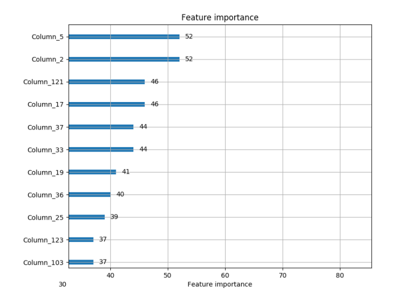
Feature Importance Plot: After running Model-1 we have listed most important features. The following figure sorts the features based on their importance:
Loss Ratio Improvement:
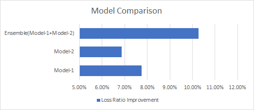
Decreased by 7.76% of current loss ratio at a reject ratio of 7%.
Model – 2
Parameters:
- ‘learning_rate’: 0.2
- ‘max_depth’: -1
- ‘max_bin’: 255
- ‘bagging_freq’ = 1,
- ‘objective’: ‘regression’
- ‘feature_fraction’: 0.5
- ‘num_leaves’:128
- ‘lambda_l1’: 1
- ‘min_data’: 20
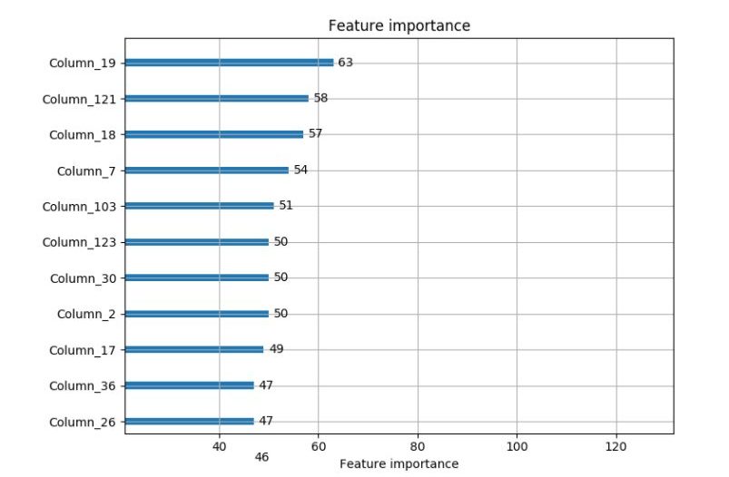
Feature Importance Plot: After running Model-2 we have listed most important features. The following figure sorts the features based on their importance:
Loss Ratio Improvement:
Decreased by 6.87% of current loss ratio at a reject ratio of 6.5%
Blending Predictions
Before blending different model predictions, there are some preprocess steps need to be checked.
Preprocess
For blending different predictions, we’ll use a simple weighted average. But before averaging them, there are some points that need to be considered. At first, predictions of the first model have come in the range of (0.000048 – 0.000891); however, the predictions of the second one are in a range o (0.0082 – 0.5622). Thus, if we do apply averaging without standardizing those predictions into the same scale, it’s highly expected that the order of the second model predictions won’t be affected by the operation.
Standardization can be applied by using the minimum and maximum value of the sets and the following formula.
min = prediction_list.min()
max = prediction_list.max()
prediction_list = (prediction_list – min) / (max – min)
After applying steps above, we’ve obtained two different prediction sets having quite similar ranges. Moreover, we’ve applied the same standardization onto validation folds by using training min and max values as well in order to avoid the potential leaks.
Another point that we need to consider is the correlation between those predictions. The lower the correlation, the higher the blending improvement. Let’s check mean correlation of each validation fold predictions.
In[40]: np.mean(correlation_list)
Out[40]: 0.5783084323078838
It’s ~0.58, which is great because it’s a quite low correlation for two different models even they provide an approximately same result. This means, there is still room to improve loss ratio by leveraging both predictions as both models were better at predicting different parts of the data.
Taking Weighted Average
Taking weighted average can be done by using following formula:
Weight = 0.5
blended_predictions = Weight*predictions_1+ (1 – Weight)*predictions_2
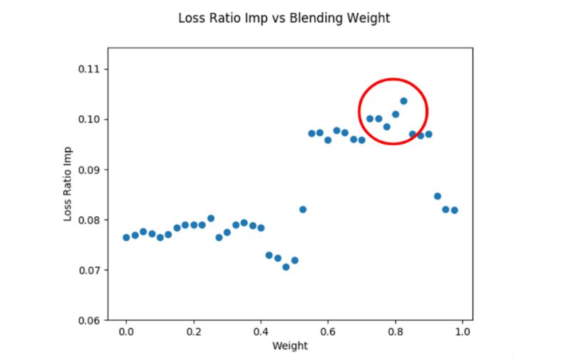
Also, you can change the weight manually and see the direction in which results change. Thanks to a “for loop”, you can generate weight values between 0 and 1 and you can simply find the weight in which the result is optimized.
As you can see on the scatter plot above, our loss ratio improvement is maximized at around 0.80 weight.
Results
With Weight = 0.7
Loss Ratio Improvement = 9.53% decrease at a reject ratio of 6.8%.
With Weight = 0.9
Loss Ratio Improvement = 9.75% decrease at a reject ratio of 6.9%.
With Weight = 0.83
Loss Ratio Improvement = 10.26% decrease at a reject ratio of 7%.
Conclusion
As you can see in the feature importance figures above, top features used during modeling are quite different from each other. Moreover, we had two different model predictions having a low correlation between them and they provided nearly same loss ratio improvement on their own. All these three statements are the sign of an upcoming improvement after ensembling.
We practiced simple weighted average on same validation predictions and obtained a significant loss ratio improvement by simply blending them. For future work, stacking can be tried as another ensembling method.
To learn more and quickly leverage what we’ve already successfully deployed for our carrier partners contact us at [email protected].